Data components

Data nodes have blue title bars and live under + Data. None of them draws anything: they produce the datasets and files that the chart and molecular components consume.

Dataset

Reads one of the project’s data files. This is usually the first node you add, because every chart needs one.

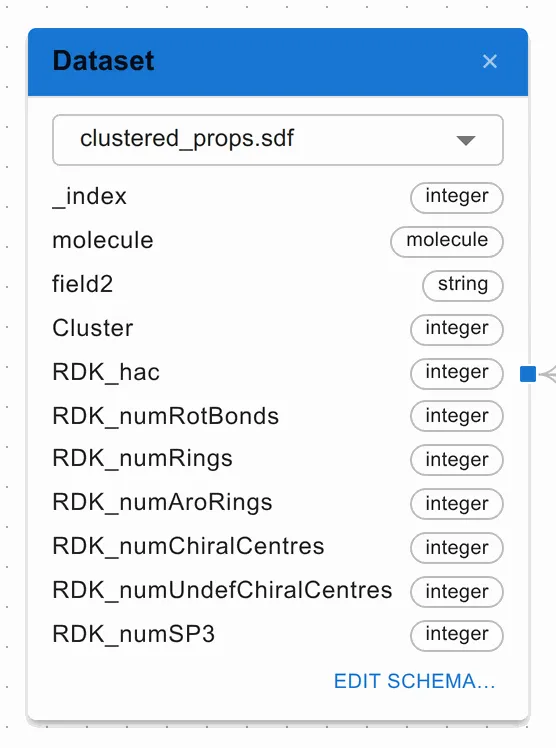
Pick a file from the dropdown. The application scans it — a spinner shows while it does — and then lists the fields it found with the type it inferred for each: integer, float, string, or molecule for a column holding structures.

Those types matter, because they decide what each field can be used for. Only numeric fields are offered as axes; only a molecule field can be a structure field. Where the scan gets one wrong — a compound identifier made of digits that should be treated as a label — Edit schema… corrects it.

Output: dataset.

Data Joiner

Combines two or more datasets into one, matching rows on a key column, so a chart can draw on columns from several files at once.

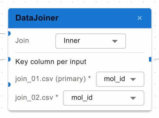
Connect each dataset to one of the joiner’s inputs; a spare input appears each time, so you can keep adding. Then choose:

• Join — Inner keeps only rows that matched, Left outer keeps every row of the first input, Full outer keeps everything from both.
• A key column for each input — the column whose values are matched.

The first input connected is marked (primary): its rows lead, and where two inputs have a column of the same name the other one is prefixed with its node’s name to keep them apart. That is a good reason to rename your dataset nodes.

Inputs: dataset × N. Output: dataset.

Calculated Fields

Adds columns worked out row by row from the columns already there. Put it between a dataset (or a joiner) and whatever comes after, and every chart downstream offers the new columns as if they had been in the file.

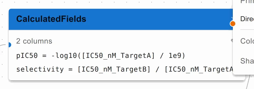
Click the ✎ to open the editor and + Add column for each one.

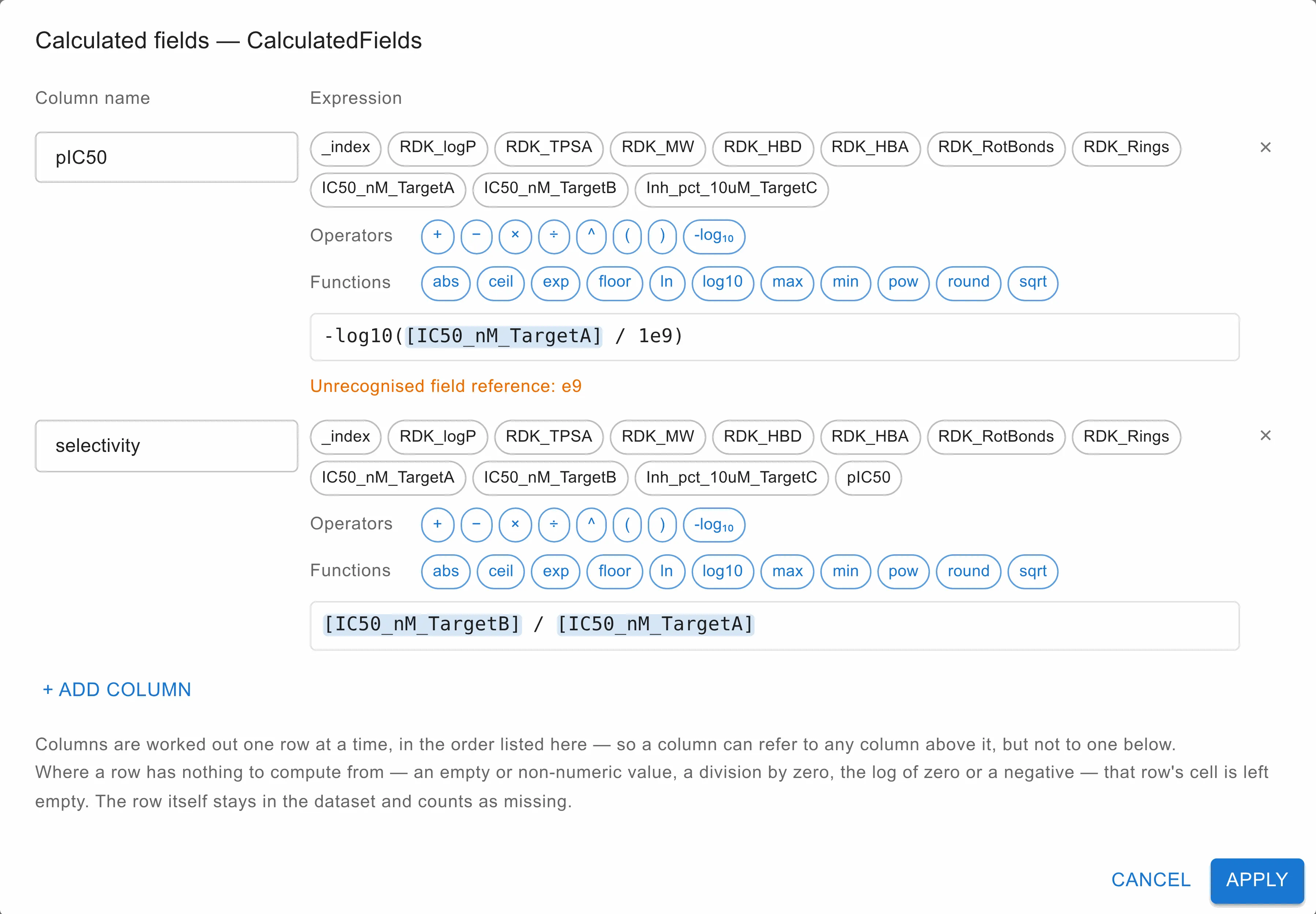
Click a field name to insert it, or type it; the operators + − × ÷ ^ and the functions abs, ceil, exp, floor, ln, log10, max, min, pow, round, sqrt are all there as buttons, and hovering one explains it.

Two things are worth knowing:

• Columns can build on each other, in the order listed. selectivity may refer to pIC50 if pIC50 is above it; the other way round is reported as an error, with a note to move it up.
• A value that cannot be worked out leaves that cell blank — a missing or non-numeric input, a division by zero, the log of zero or a negative. The row stays in the dataset and counts towards the chart’s missing figure. An expression that does not parse, by contrast, adds no column at all and says what is wrong: a whole column of blanks would look like a problem with your data rather than with the expression.

Note that ^ binds more tightly than a leading minus, so -2^2 is -4 — the mathematical convention, which differs from Excel’s.

The transform adds columns and changes nothing else: same rows, same order, so selections and filters wired across it keep working. Nodes chain, and work after a joiner as well as after a file.

Input: dataset. Output: dataset.

FileSelector

Supplies structure files — a receptor, a reference structure — to the nodes that need one. It is the only way a protein reaches the 3D viewer or either of the interaction views.

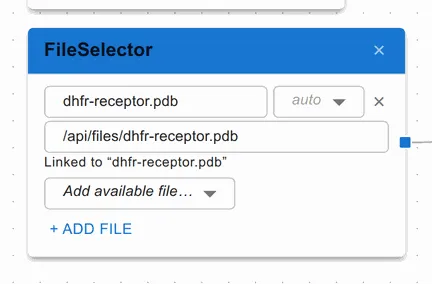
Pick from Add available file… and the entry is linked to that project file. A linked entry says so, and is re-resolved against the project each time the visualisation is loaded — which is what lets a saved visualisation work in a new instance, whose internal addresses are different. Typing a location by hand instead is allowed, but unlinks the entry.

If a linked file is no longer in the project, the node says so rather than silently doing nothing.

Output: files. A MoleculeViewer3D loads every file on the port; the two interaction views use the first as their receptor.