Molecular components

Molecular nodes have green title bars and live under + Molecular. Most need a field holding a molecule — the structure column of an SDF file, or a SMILES column — chosen on the node in the Design tab.

Two of them need something more: a protein structure, which reaches them through a FileSelector, and a sketched structure, which comes from a MoleculeSketcher.

The 3D viewer and the two interaction views take some of their settings from named presets. A preset is defined once for the whole project and shared by every chart that names it, so the three views of the same poses cannot disagree about what counts as a contact.

MoleculeCardGrid

A paginated grid of 2D depictions, each with the property values you asked for underneath — as text, or as a small bar chart or radar plot.

Fields: Structure*, Display fields.

Tab	Settings
Appearance	How the display fields are drawn (text, bar chart or radar), molecule size, force 2D, SDF export format
Layout	Cards per page, sort by, only selected
Algorithm	Require filter, then the structure search

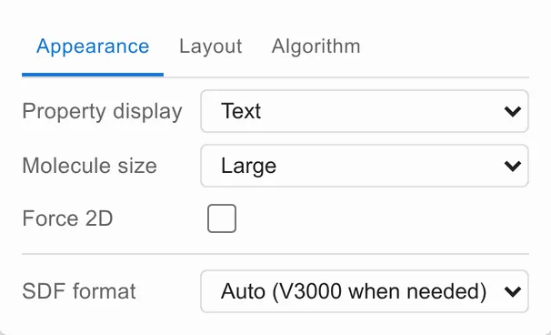
Require filter is on by default and matters: drawing a depiction is real work, and a grid pointed at ten thousand molecules with nothing filtering it would take a long time. Leave it on and wire a selection into the grid’s filter port; turn it off only for a dataset you know is small.

Force 2D redraws a molecule that carries 3D coordinates as a proper flat depiction, instead of projecting its 3D geometry onto the page — which is usually what you want for a docking pose.

Structure search filters the grid by a structure drawn in a MoleculeSketcher wired into its molecule port. Substructure keeps molecules containing the sketch; Similarity keeps those above a threshold you set. In substructure mode the matched part is shaded and each hit is oriented the way you drew the query, so the series lines up — both can be switched off.

Right-clicking a card offers Copy molecule, Copy as SMILES, Copy as CXSmiles, Copy as PNG and Download PNG.

MoleculeSketcher

An embedded structure editor. It has no data input: you draw in it, and what you draw goes out of its molecule port to a MoleculeCardGrid (as a search query) or an RGroupTable (as the core scaffold).

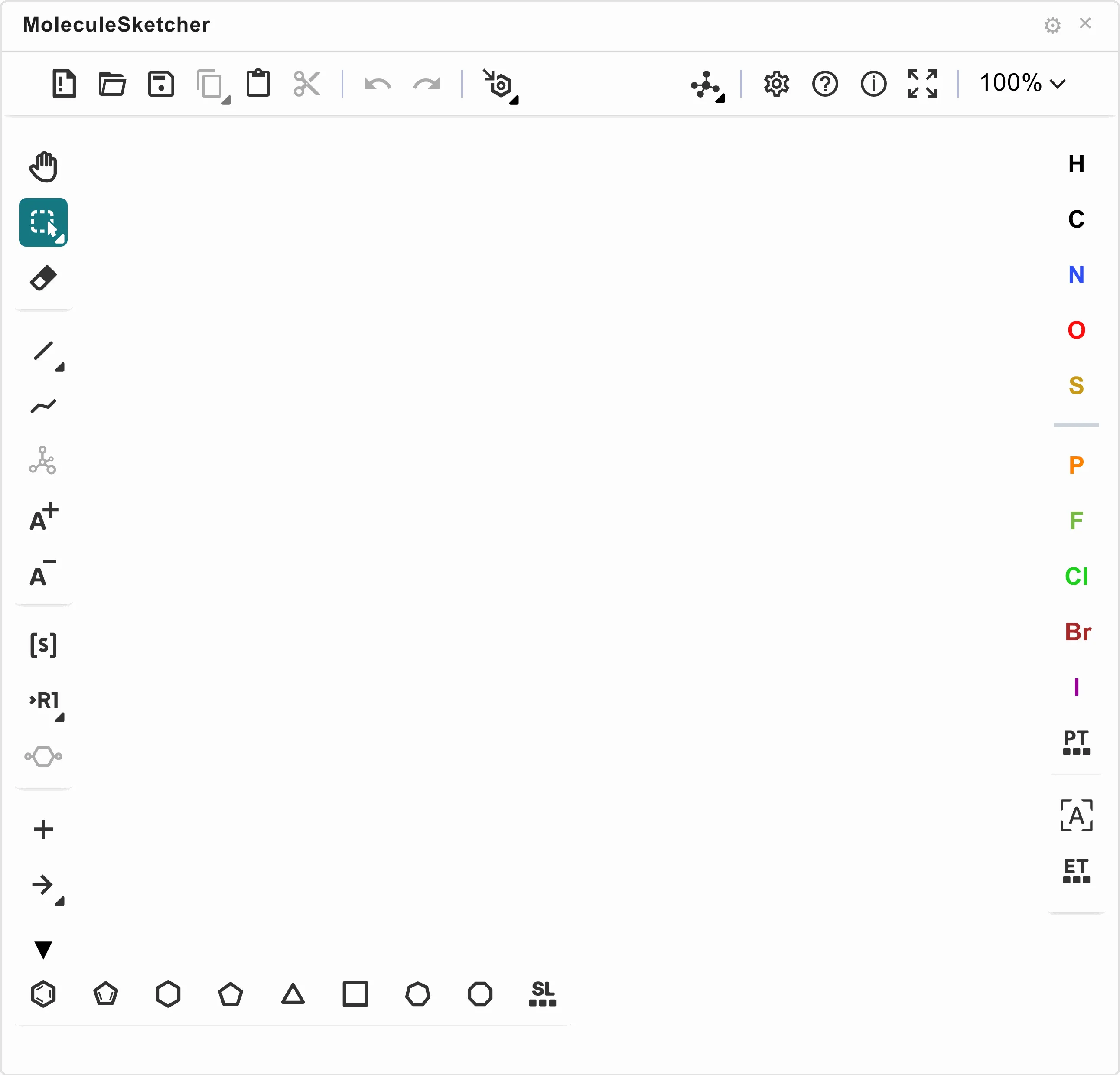
Its ⚙ chooses what you are drawing, which changes what the editor offers:

Mode	For
Default	The editor exactly as it ships
Query	A substructure query — generic atoms, R-groups and query fields stay available, and valence warnings are off, since a partial query legitimately has odd valences
Molecule	A real molecule — the generic-atom and R-group tools are removed and implicit hydrogens are labelled

Switching between query and molecule rebuilds the editor, which takes about a second; whatever is on the canvas is carried across.

What you have drawn is not saved with the visualisation. Loading a saved visualisation gives you the wiring and the settings, but an empty sketcher — so the grid or table it feeds will ask for a structure again.

RGroupTable

Decomposes a set of molecules against a core scaffold and lays the substituents out as a table: one R-group down the side, another across the top, and the molecules carrying that combination in each cell.

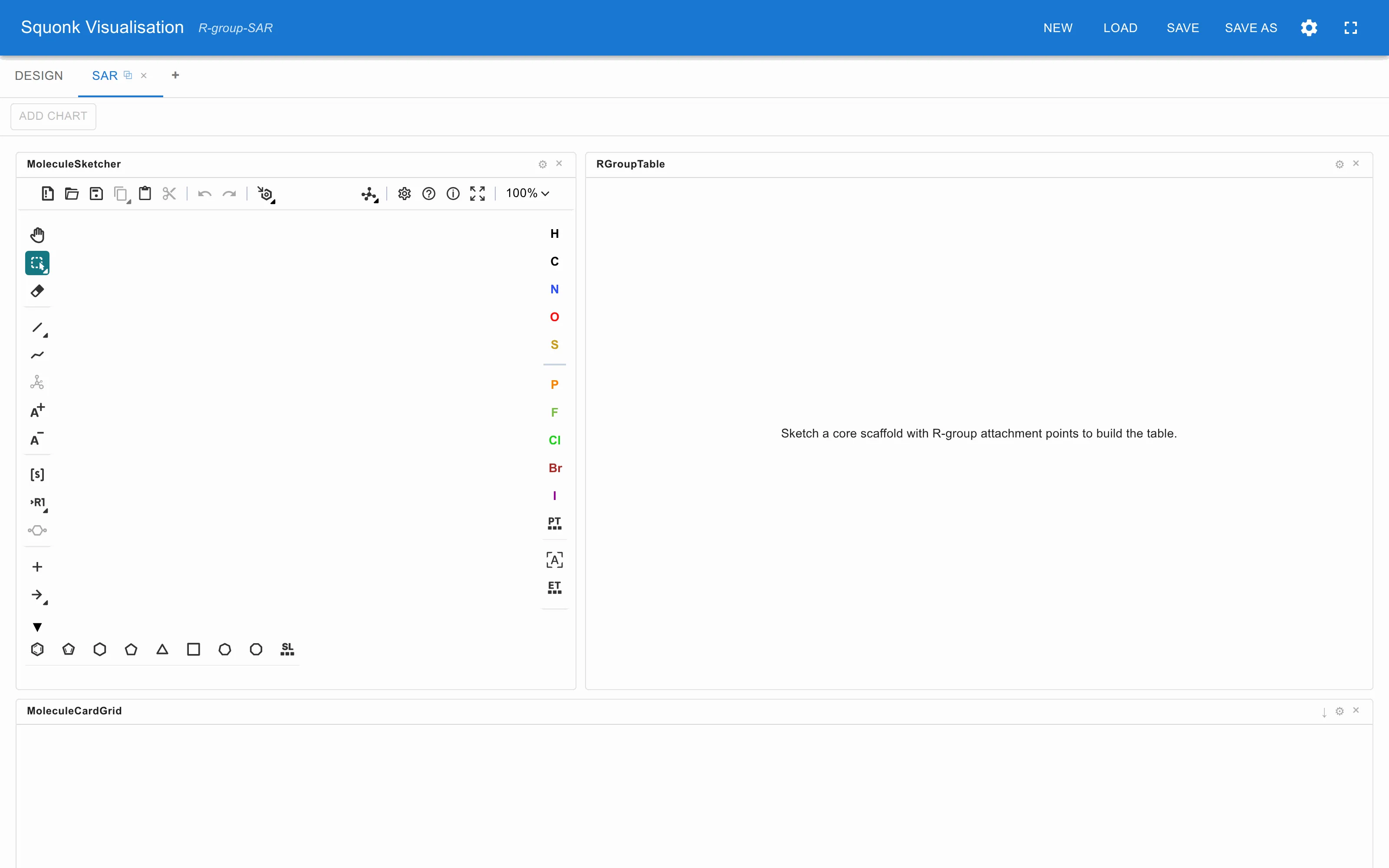
Fields: Structure*, Label, Cell fields.

Set it up like this:

1. Add a MoleculeSketcher and wire its molecule output to the table’s Scaffold input.
2. Wire a Dataset to the table’s dataset input, and choose the structure field, a Label field naming the molecule in each cell, and the Cell fields to show.
3. In the sketcher, draw the core with R-group attachment points — the R1 tool in the left-hand toolbar. Until you do, the table says so, as above.

Draw the scaffold; do not open it from a file. Ketcher’s own Open structure dialog will put a structure on the canvas, but the sketcher only publishes what you draw, so the table will carry on asking for a scaffold that is plainly on screen. The same applies to the structure search on MoleculeCardGrid.

In the ⚙: which R-groups form the Rows and Columns (a scaffold with three or more R-groups collapses the rest into the cell), and what each cell shows — Text, Bar chart, Radar, or Structure for a 2D depiction.

In Structure mode every molecule is drawn in the same orientation as the sketch, so the shared core is the same way up in every cell — which is the comparison the table exists to make. The substituents are shaded rather than the core, because the core is the same everywhere and shading it would cover most of the picture.

MutationShells

A radial view of a series. One molecule sits at the centre as the anchor and every other is placed on a concentric ring by how many edits separate it structurally from that anchor, with a side plot of the property you are optimising.

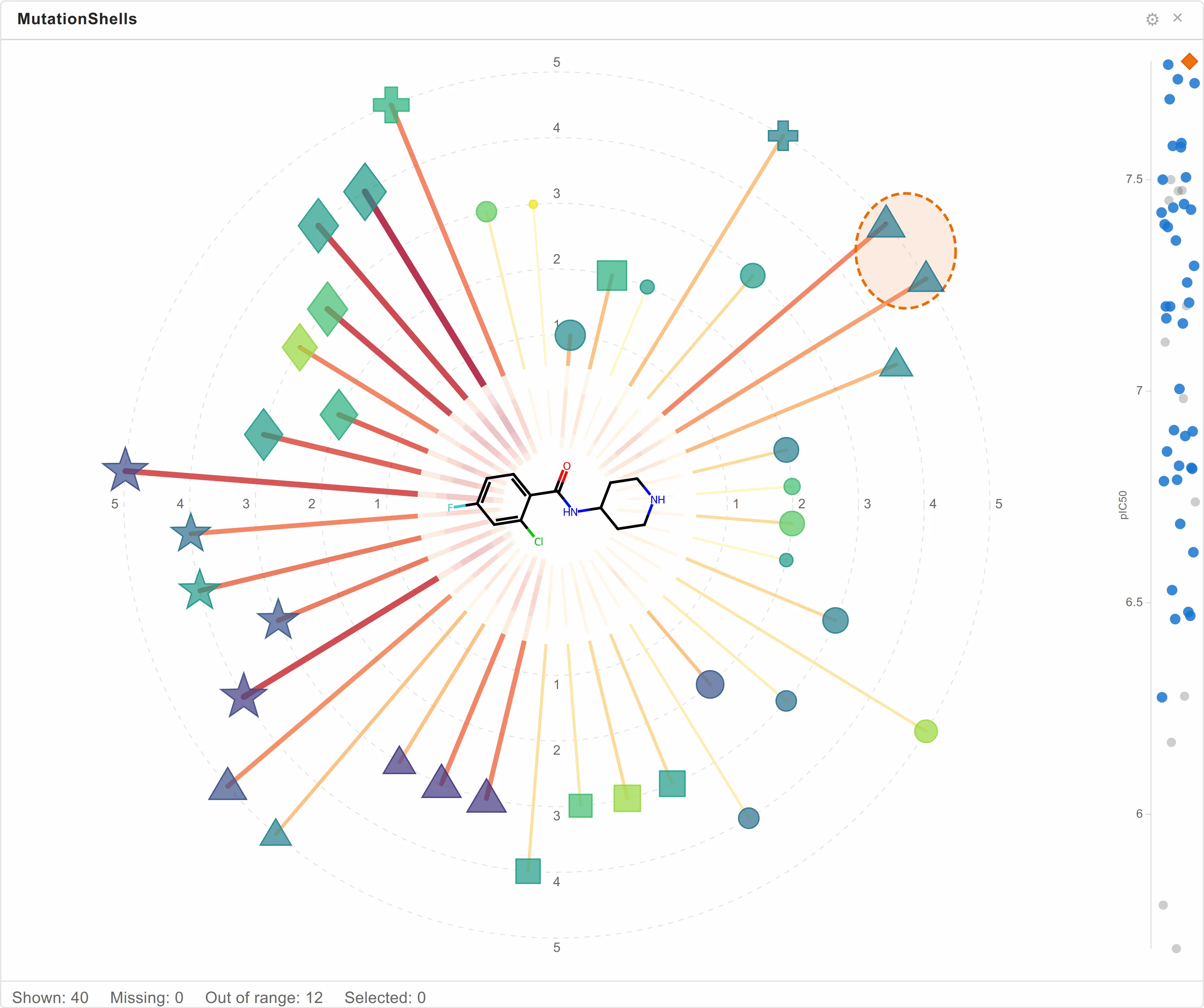
Fields: Structure*, Primary* (with a direction saying which end is best), Colour by, Shape by.

The anchor starts as the best-scoring row; click another glyph, or a point in the side plot, to re-anchor, and use the Back / Forward buttons to retrace.

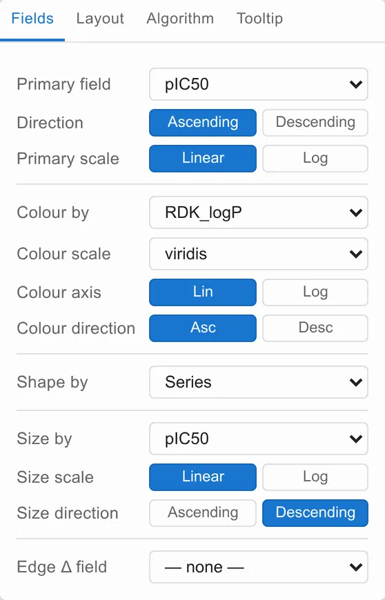
Its ⚙ has four tabs — Fields, Layout, Algorithm, Tooltip. Layout sets how many rings to draw and how the glyphs are spread around them; Algorithm sets the cost of each kind of edit (adding an atom, changing an element, changing a bond order, inverting a stereocentre), which is what decides which ring a molecule lands on.

The distances take a moment to compute, and a progress indicator shows while they do.

MoleculeViewer3D

An interactive 3D view of ligands, optionally inside a protein. It is built on NGL Viewer, so the representations, colour schemes and mouse controls are NGL’s.

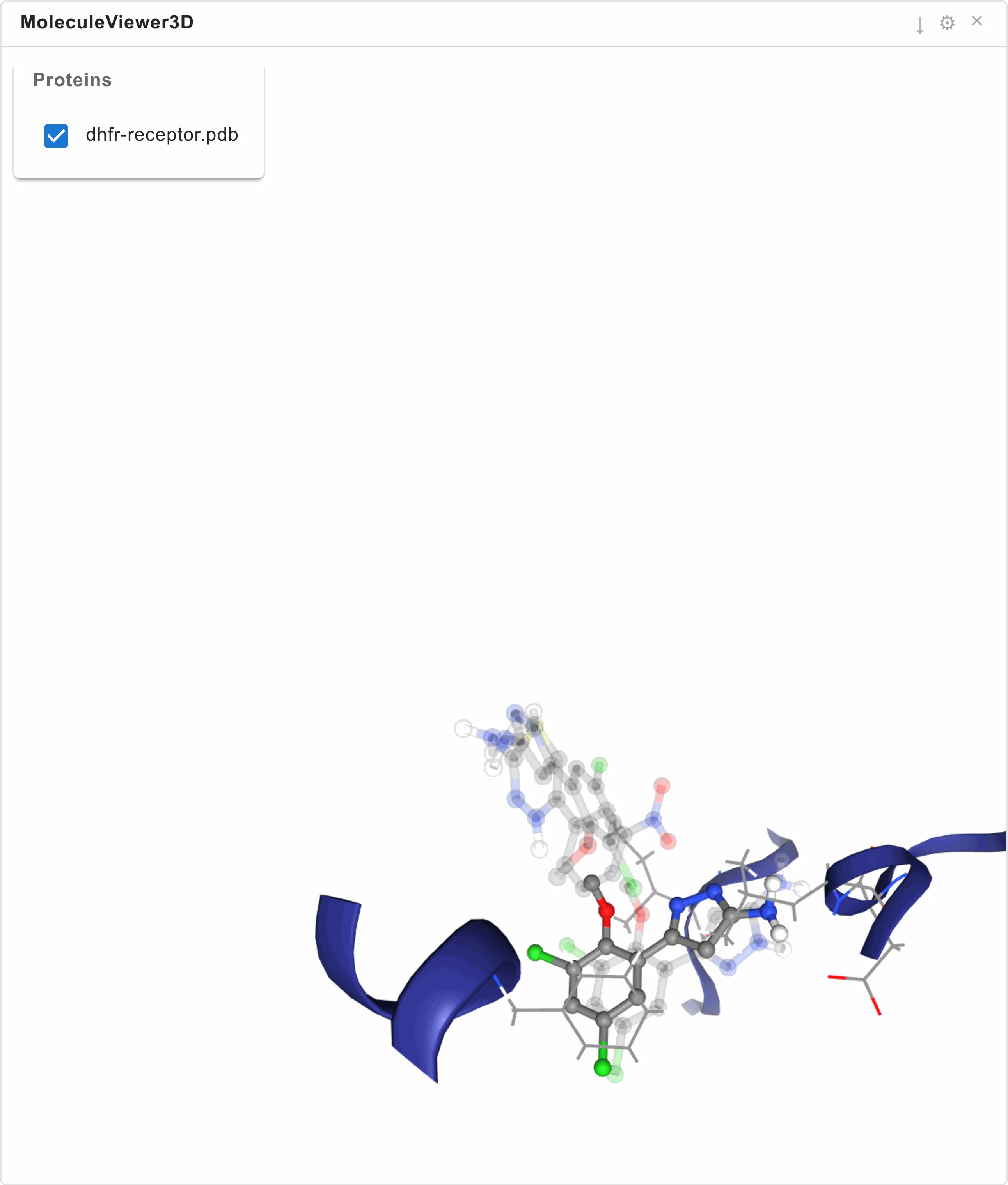
Fields: Molecule field* (a 3D structure).

Wire a FileSelector to its files port to load proteins — it loads all of them — and a dataset to its dataset port for the ligands. A panel in the viewer’s top-left corner lists the proteins with a checkbox each.

Action	How
Rotate	Drag with the left button
Zoom	Scroll
Pan	Drag with the right button
Inspect an atom	Hover it

Tab	Settings
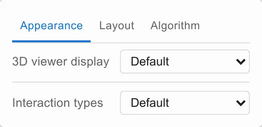
Appearance	The 3D viewer display preset and the Interaction types preset
Layout	Whether the Proteins panel is shown, and Show only highlighted residues
Algorithm	Require filter, Show interactions, and the Interaction cutoffs preset

The viewer has no ligand or protein style settings of its own. They all come from the 3D viewer display preset it names. To change how it draws, make a preset under Settings → Presets and pick it here.

Three things are worth understanding here.

Filter and marking do different jobs. The filter port decides which ligands are loaded at all; marking decides which of those stand out, the rest being dimmed rather than removed. Sending a shortlist to the filter and the pose you are looking at to the marking is how you keep the context and still see the one.

Show interactions overlays the detected ligand–protein contacts as dashed lines, coloured by type, using NGL’s own live contact detection — the same feature the standard NGL web application offers. The colours match the 2D interaction diagram, so a contact is the same colour in both.

Show only highlighted residues hides the rest of the protein and draws only the residues arriving on the highlightResidues port, which is how you get from a whole fold to the binding site. It does nothing until something is wired into that port, and the setting says so until then. Note that the ribbon and surface overlays follow the region around those residues rather than the residues themselves — a cartoon needs a continuous run of backbone to draw at all, so it is given a couple of residues either side.

LigandInteractionMap

What each ligand actually touches, as a grid: one row per ligand, one column per residue.

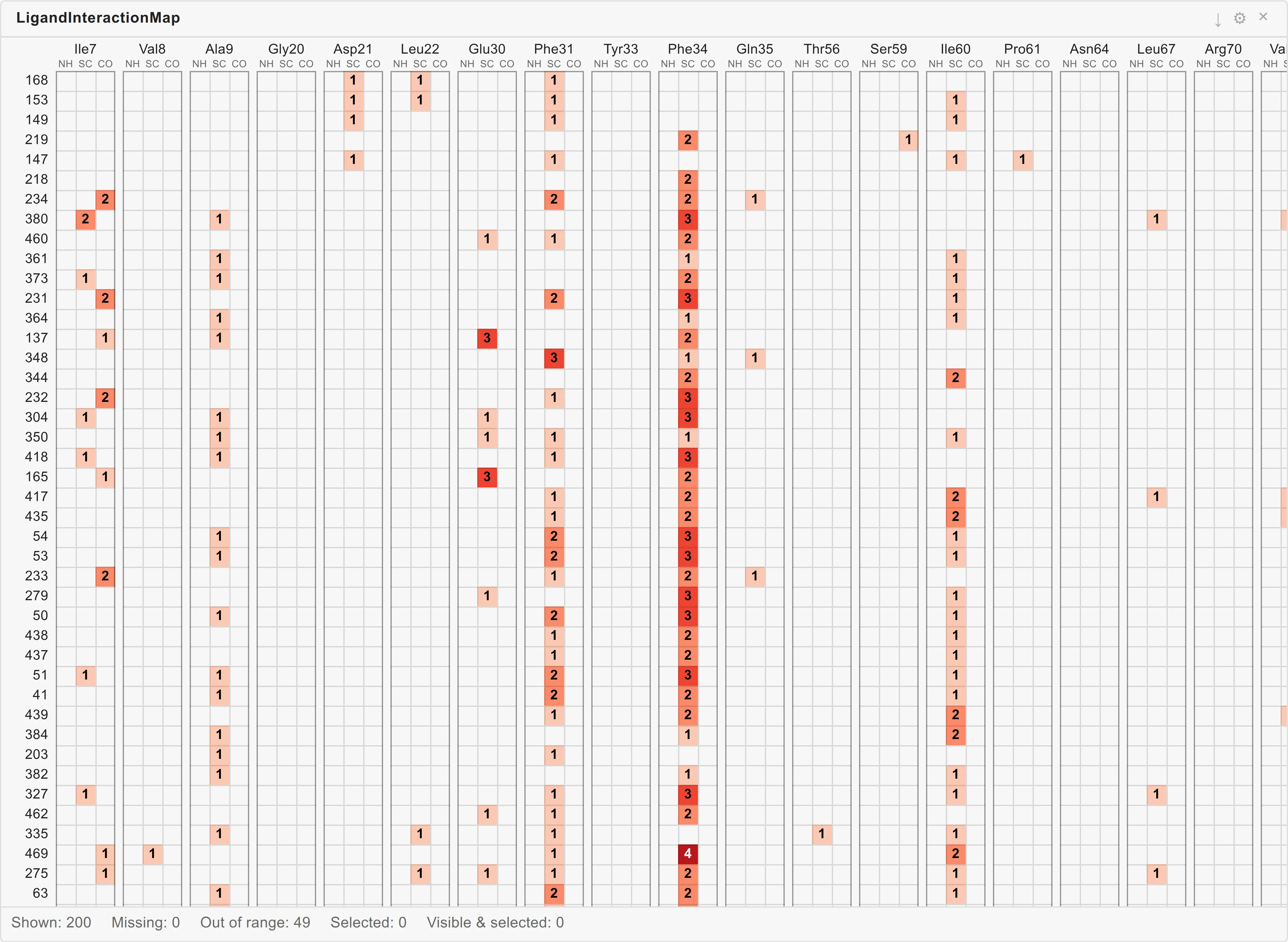
Fields: Ligand field* (3D poses), Row label, Sort by.

Every residue is three sub-boxes — backbone N–H, sidechain, backbone C=O, left to right, following the residue’s own N–Cα–C order — so you can see which part of a residue is engaged, not only that it is. The number of interactions is printed in each, on a fixed red scale, so a shade means the same thing in every chart and no legend is needed. Empty sub-boxes stay blank.

The contacts are detected by NGL, using its own interaction engine — the same code behind NGL’s “contact” representation, run without a 3D canvas. Ten types are recognised: H-bond, backbone H-bond, weak H-bond, water H-bond, hydrophobic, π-stacking, cation-π, ionic, halogen bond and metal coordination.

Setting it up:

1. Wire a Dataset whose molecule field holds 3D poses to its dataset port.
2. Wire a FileSelector holding the receptor to its files port. It uses the first file there.
3. Choose the Ligand field, and optionally a Row label and a numeric Sort by field on the node.
4. Wire a selection into its filter port. Nothing is computed until you do.

The poses and the receptor must be in the same coordinate frame — the poses as docked into that receptor. Poses from a different copy of the protein produce no contacts at all, and the map will simply be empty.

Using it:

• Click a cell to select that ligand, replacing the selection. Drag vertically to select a range; shift-drag adds to the selection.
• Click a ligand’s name in the left-hand gutter to toggle just that ligand in or out — no modifier needed, which is how you build up a shortlist one click at a time.
• Click a residue’s NH / SC / CO header to filter the rows to ligands with an interaction there. Selecting several combines them with and. Click again to clear one, or Escape to clear everything.
• Hover a sub-box to see exactly which atoms are involved.
• Both label bands stay pinned as you scroll, like a spreadsheet’s frozen row and column, so a cell deep in a large grid can always be read off against both.

Tab	Settings
Appearance	The Interaction types preset, and cell size
Axes	Residue order (sequence or most-contacted first), the minimum number of ligands a residue needs to earn a column, and the ligand sort direction
Algorithm	Require filter, Max ligands, and the Interaction cutoffs preset
Tooltip	What hovering a ligand’s name shows — name a molecule field to draw its structure

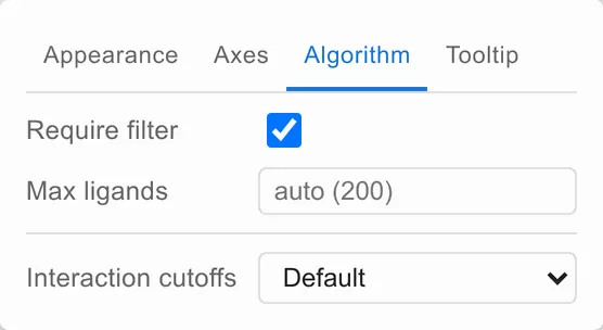
Detection costs roughly 40 ms per ligand, which is why Require filter is on by default and why Max ligands caps the run at 200. Rows past the cap are counted as out of range. Changing the interaction types is free — every type is detected in one pass, and the setting only filters what is shown — whereas changing the cutoffs re-runs the detection. Both are presets, shared with the diagram and the 3D viewer.

LigandInteractionDiagram

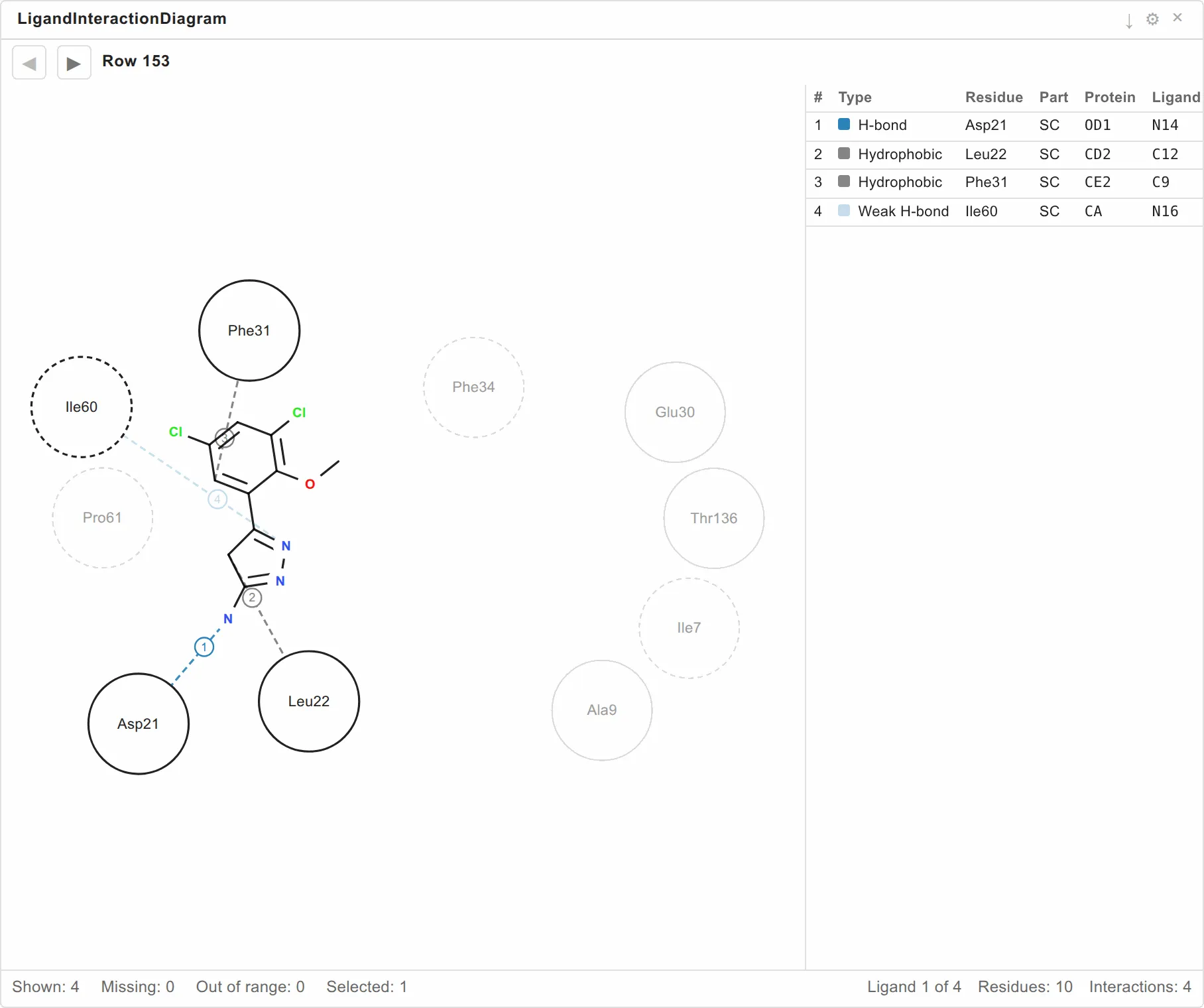
The same detected interactions — the same NGL engine, the same cutoffs — drawn as a flat diagram: the ligand as a 2D structure, ringed by the residues it contacts, one dashed line per interaction coloured by type, and a numbered table of them beside it — one row per line drawn, giving its type, the residue and which part of it, the two atoms involved and the distance between them.

Fields: Ligand field*, Panel title, Navigate by.

It is set up exactly like the map — dataset, receptor on the files port, and a filter — and shows one ligand at a time, stepped through with ◀ ▶ or the ← → arrow keys while the panel has focus.

How the layout is worked out

Briefly, because it explains what the picture can and cannot tell you:

1. A plane is fitted through the binding site and everything is projected onto it. How far a residue lies in front of or behind that plane becomes the depth cue on its bubble.
2. Residues are placed at their projected angle around the ligand’s centre, pushed out clear of the ligand, then nudged apart until they stop overlapping — keeping each one’s direction while relaxing its distance. So the angle around the ligand is meaningful; the distance is not.
3. The ligand is drawn as a clean 2D depiction and rigid-fitted onto its own projected pose, so its orientation follows the real 3D pose rather than a drawing convention. That is the default; the alternative is below.
4. The residue positions are computed once, for the whole set — every ligand admitted by the filter — not per ligand.

That last point is what makes the view worth having. Stepping from one ligand to the next changes the ligand, its lines, and which residues are live, and nothing else. A residue drawn pale has been lost by this ligand, not moved, so two poses can be compared across a step from memory.

Because a flat drawing of a deep pocket can put two distant residues on top of each other, the layout is scored, and when it is poor the status bar carries a warning naming the offending pair. It never blocks the drawing.

Two ways to draw the ligand

Ligand geometry, on the Appearance tab, chooses between them. They answer different questions and neither is right for both.

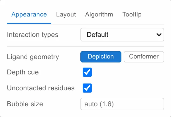
Depiction — the default — draws a clean 2D structure of the molecule and then rotates, mirrors and scales it as a rigid whole onto the pose’s own projection.

Conformer draws the pose’s own coordinates, flattened onto the same plane — the molecule exactly as the projection sees it.

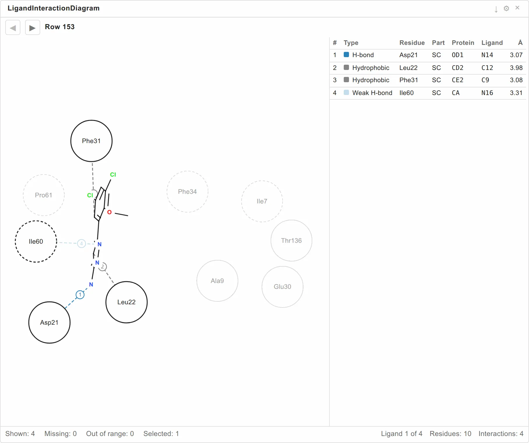
Both pictures above are the same pose, with the same four interactions to the same residues. The difference is what has been idealised:

	Depiction	Conformer
Chemistry	Readable — rings look like rings, bond lengths and angles are regular	Depends on the pose. Where the molecule lies flat in the projection plane it reads perfectly well; where it folds towards you, a ring can collapse to a line and bonds overlap
Atom positions	Approximate. The drawing is fitted onto the projection as a whole, so an atom is near where it really is, not on it	Exact. Every atom is precisely where the projection puts it
Conformation	Smoothed away. A strained or unusual conformation is drawn as the idealised molecule	Preserved, including whatever is odd about it
Orientation	Follows the real 3D pose — the fit decides which way up it goes	Follows the real 3D pose, by construction

Do not read too much into the two pictures above. They are one pose out of a set, and this one happens to project badly — it folds towards the viewer, so Conformer flattens two of its rings into near-lines. That contrast is why it was chosen to illustrate the setting, not evidence that Conformer usually looks like this. A ligand that lies roughly in the projection plane, or a smaller or more rigid one, can come out perfectly readable — and then Conformer gives you readability and exact positions, which is strictly more than Depiction offers.

Which to use is worth deciding per pose rather than once. Depiction is the safe default because it is readable whatever the pose does. Conformer is the better picture whenever it is legible, and is the one to reach for when you need to judge exactly which atom faces which residue, when you are checking that an odd-looking fit is the pose and not the drawing, or when the conformation itself is the point — a folded or strained ligand is precisely what Depiction smooths away. Flipping between the two on the same pose costs nothing, so it is worth a look.

Stereochemistry survives either way: when the fit mirrors the depiction, its wedge and hash bonds are flipped to compensate, so a mirrored layout does not silently invert a stereocentre.

One thing to expect when you switch: the residue bubbles shift a little. They are placed clear of the ligand’s footprint, and the two geometries have different footprints. Within one setting the stage is still fixed across the whole set, which is what stepping between ligands relies on.

Tab	Settings
Appearance	The Interaction types preset, ligand geometry, whether residues behind the plane are dashed, whether uncontacted residues are drawn, and bubble size
Layout	Max residues, Panels, where the interaction table goes, and whether the ◀ ▶ buttons are shown
Algorithm	Require filter, Max ligands, the Interaction cutoffs preset
Tooltip	The tooltip expression

The Interaction types and Interaction cutoffs rows pick presets, the same ones the map and the 3D viewer use.

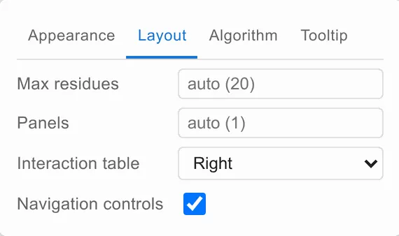
Panels draws several diagrams side by side, each stepped independently against the same residue positions — the same comparison, without having to hold the previous ligand in your head. Panels are never drawn below a readable size; ask for more than fit and the grid scrolls.

Max residues caps how many residues are drawn, because past about thirty the diagram stops being readable. Residues dropped by the cap take their interactions with them, so the status bar counts them and a warning names them.

Hovering a line tints its table row and vice versa; hovering a residue highlights everything involving it. Clicking pins the highlight so the pointer can leave, and Escape releases it.

What it reports: the ligand each panel is showing is this view’s selection, so wiring its selection output to a 3D viewer’s marking follows your navigation in 3D. Its residues output reports what those ligands contact, for the viewer’s highlightResidues.